CS205 Final Project

Cooper Lorsung • Sujay Thakur • Royce Yap • David Zheng

Introduction Overview Big Data Big Compute Results and Discussion Citations

Overview

Problem

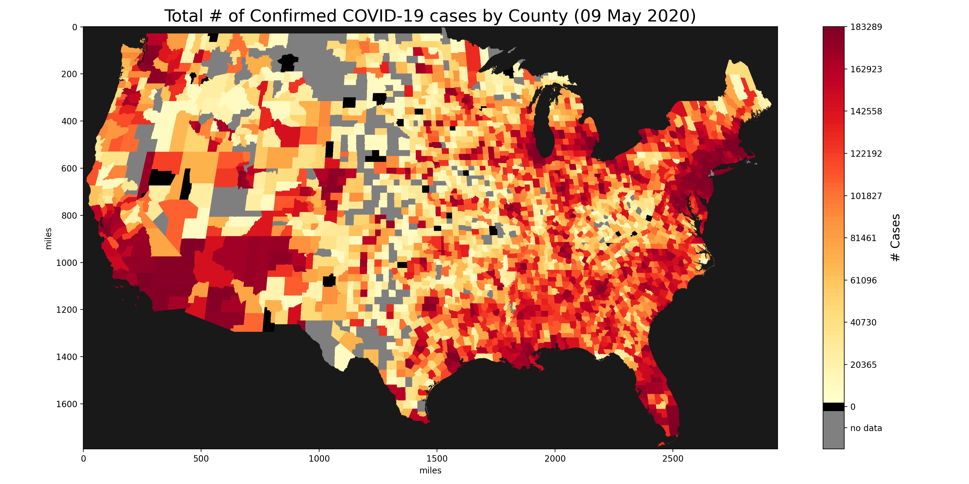
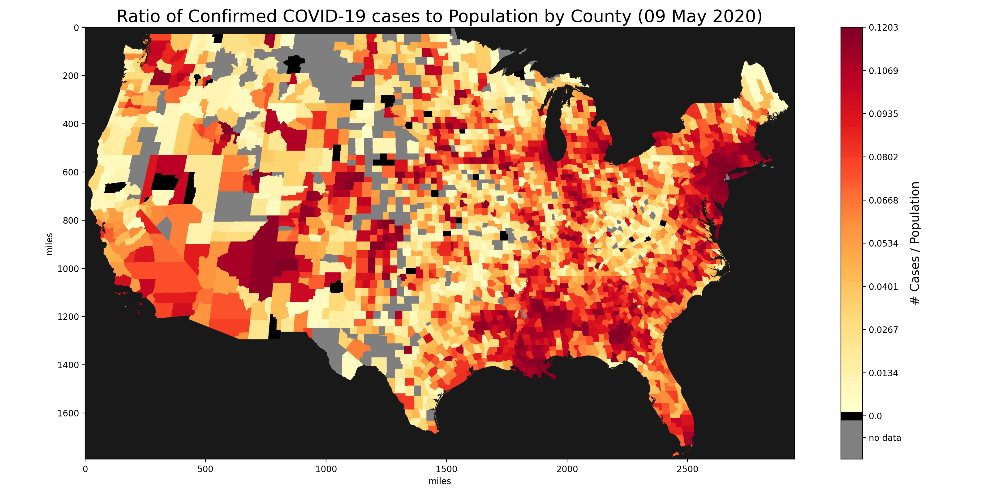
Images generated from our matrix with data aggregated from the US Census Bureau, Johns Hopkins University and the New York Times.

The global pandemic of COVID-19 has gripped the world causing significant changes in day-to-day life for a huge number of people. With any disease, and especially ones as dangerous as this one, it is important to understand how it spreads. Many models and projections exist already, but they are mostly on a coarse national/state scale. It is difficult for local authorities to fully understand the spread in their immediate regions and hence craft carefully-tailored policies.

Solution

We use a mechanistic model to help better understand the spread of COVID-19. We aim to generate projections on a more granular scale than current models. This empowers regional authorities to tailor containment measures to their demographic, rather than base policies on projections that are on a larger scale.

In order to accurately model the spread, we take a 2944×1792 grid approximation of the US and run the spatio-temporal SIR model (explained in detail below) at each point on the grid.

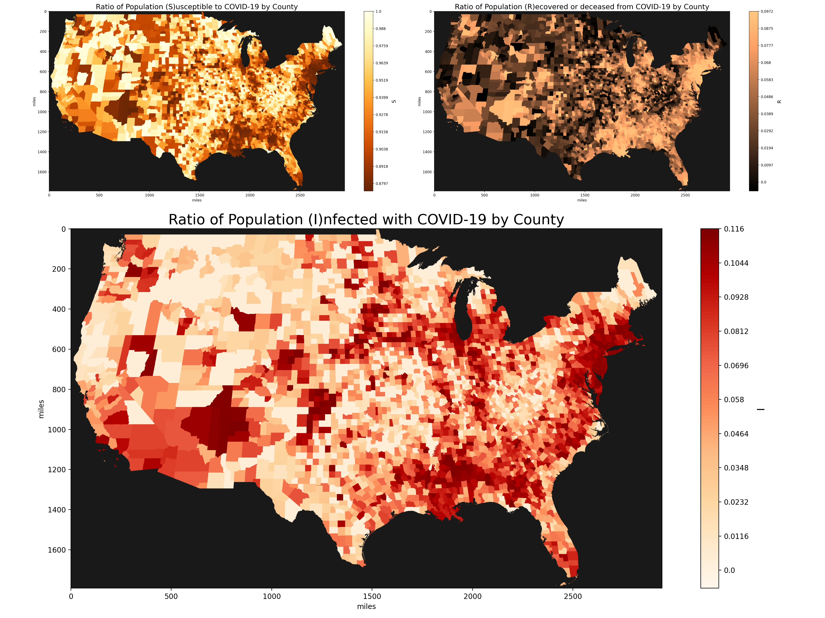
Plot of initial SIR parameters based on existing COVID-19 data.

Description of model and data

The temporal SIR model is a common epidemiological model (Chen, et.al, 2020) that tracks the number of Susceptible (S), Infected (I) and Removed (R) individuals in the population. Note that R consists of both recovered and dead people. To incorporate a spatial dimension, we use the more expressive spatio-temporal version (Lotfi, et. al, 2014) described by a set of partial differential equations:

$\frac{\partial S}{\partial t}=d_S\nabla^2S-\beta SI$
$\frac{\partial I}{\partial t}=d_I\nabla^2I+\beta SI-\gamma I$
$\frac{\partial R}{\partial t}=d_R\nabla^2R+\gamma I$

As seen, this model explicitly considers the diffusion of the infection with the Laplacian operator and hence allows for a more complex and realistic simulation. We discretize the Laplacian as follows:

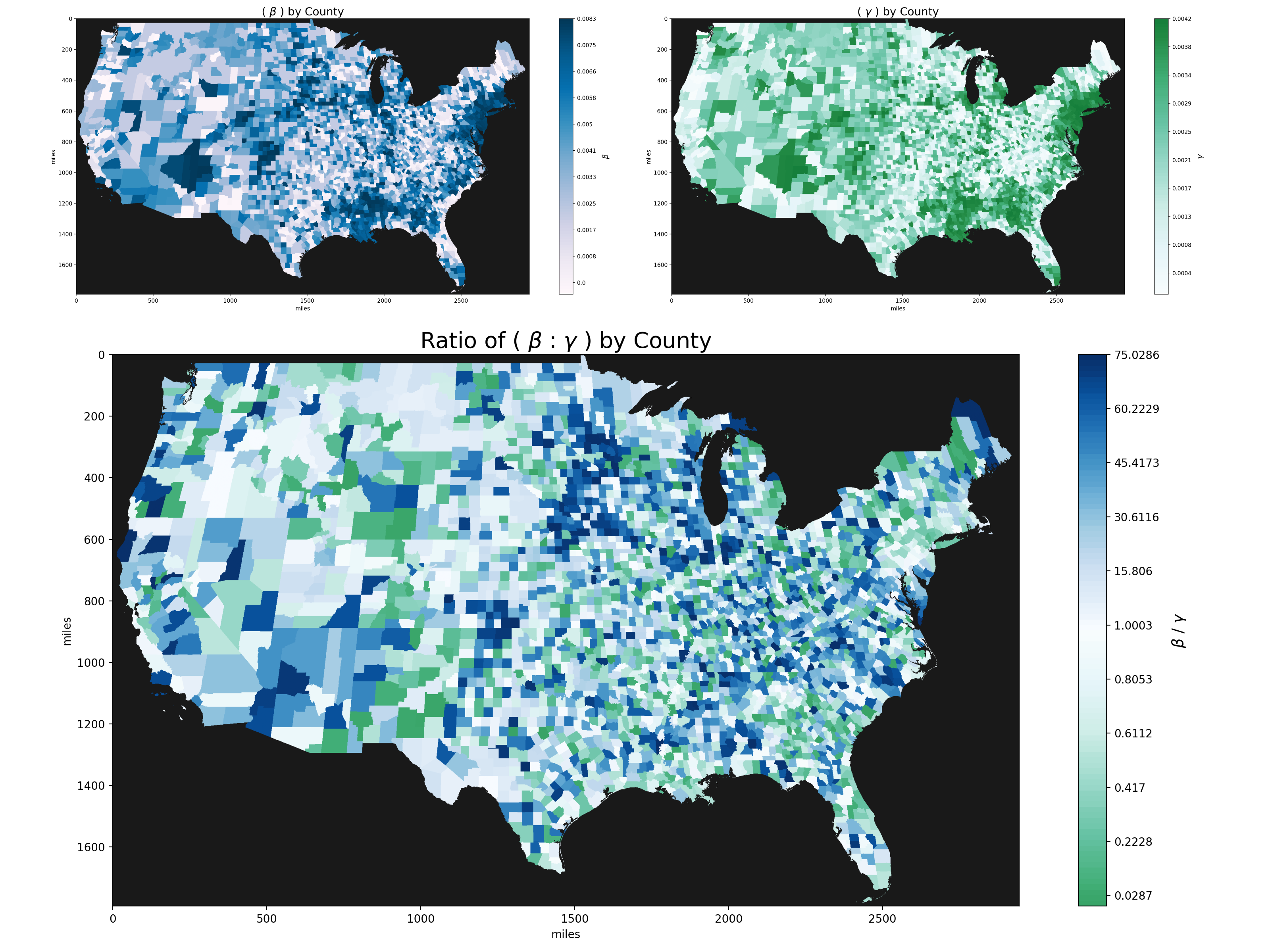
$\nabla^2S\approx\frac{S(x-\Delta x,y)+S(x+\Delta x,y)-4S(x,y)+S(x,y-\Delta y)+S(x,y+\Delta y)}{\Delta x\Delta y}$

Plot of beta and gamma hyperparameters based on a 14 day average of COVID-19 infection and recovery/death rates

In this model, β, γ, d_S, d_I, d_R describe the transmission rate, recovery rate, susceptibilty diffusion rate, infection diffusion rate and recovery diffusion rate respectively. It is common in most models to consider them as fixed. However, in order to allow for a more granular simulation, our model considers β(x,y), γ(x,y), d_S(x,y), d_I(x,y), d_R(x,y), ie we allow each parameter to be different for each grid point. This is a much more realistic description of the true underlying spread mechanism in which each local region has wildly differing characteristics. This means that we need to create 2944×1792 arrays for each of these parameters, which requires the complex processing of large amounts of granular data. This is a prime example of a problem requiring Big Data solutions.

Combining the paramater discretizations, the update steps are given by:

$S^{t+1}_{i,j}=S^{t}_{i,j}+d_{S_{i,j}}(S^t_{i+1,j}+S^t_{i-1,j}-4S^t_{i,j}+S^t_{i,j+1}+S^t_{i,j-1})-\beta_{i,j}S^{t}_{i,j}I^{t}_{i,j}$
$I^{t+1}_{i,j}=I^{t}_{i,j}+d_{I_{i,j}}(I^t_{i+1,j}+I^t_{i-1,j}-4I^t_{i,j}+I^t_{i,j+1}+I^t_{i,j-1})+\beta_{i,j}S^{t}_{i,j}I^{t}_{i,j}-\gamma_{i,j}I^{t}_{i,j}$
$R^{t+1}_{i,j}=R^{t}_{i,j}+d_{R_{i,j}}(R^t_{i+1,j}+R^t_{i-1,j}-4R^t_{i,j}+R^t_{i,j+1}+R^t_{i,j-1})+\gamma_{i,j}I^{t}_{i,j}$

Hence, in this model, for each time step at each grid point, we will be reading in spatial information for β, γ, d_S, d_I, d_R and computing the updates for S, I and R. We will do this for 2944×1792 = 5,275,648 grid points per time step. This is a prime example of a problem requiring Big Compute solutions.