CS205 Final Project
Cooper Lorsung • Sujay Thakur • Royce Yap • David Zheng
Big Compute

Description of Parallel Application
OpenMP was used to parallelize computations in our model. Loop level parallelization was done to optimize performance. Explicit memory sharing was used for parameter matrices, as well as loop collapsing. We compared execution using a single node on the Odyssey cluster against an AWS t2.2xlarge instance. Odyssey was ultimately used for its superior performance. We found sufficient speedup using one node that multiple were unnecessary.
Instructions for running on Odyssey
Required Directory Structure
In order to run on the cluster, the required directory structure is shown below:
generate_data.py
generate_plot.py
data/
|  matrix.npy
project_runs/
|  run.py
|  sir_data_omp.c
|  template.sh
|  timing.c
|  timing.h
|  plot_speedup.py
results/
matrix.npy contains granular county-level data. Download instructions are provided below. generate_data.py creates the required data CSVs from matrix.py and stores them in data/. generate_plot.py reads in the simulation output from results/output and plots them in results/output.png. run.py handles compilation and setting appropriate environment variables for number of cores. Slurm job parameters such as number of nodes, cores, runtime, and partition are updated in the __main__ section of run.py, as well as number of timesteps to simulate for. The rest of the files are the actual models.
Required Dependencies
The compiler gcc/8.2.0-fasrc1 is used. OpenMP comes prebuilt with the compiler. Python 3.7.7 is used. Runs are executed on the default Odyssey operating system at the time of submission: CentOS Linux release 7.6.1810 (Core).
Run module load python/3.7.7-fasrc01 and module load gcc/8.2.0-fasrc01 to get the required dependencies.
Running the simulation tools
- Use this link and download
matrix.npyinto thedata/subdirectory. - Run
python3 generate_data.py(might take ~1 min) to create the required data CSVs that will be placed in thedata/subdirectory. - Run
python run.pyfromproject_runs/. - Run
python3 generate_plot.pyfrom the main directory to create a visualization of the simulation result asresults/output.png.
Instructions for running on AWS
Required Directory Structure
In order to run on AWS, the required directory structure is shown below:
generate_data.py
generate_plot.py
data/
|  matrix.npy
models/
|  sir_data_omp.c
|  sir_data.c
results/
matrix.npy contains granular county-level data. Download instructions are provided below. generate_data.py creates the required data CSVs from matrix.py and stores them in data/. generate_plot.py reads in the simulation output from results/output and plots them in results/output.png .The rest of the files are the actual models.
Required Dependencies
We recommend running on an AWS t2.2xlarge instance with Ubuntu 16.04. Python 3.7.7 was used, with numpy and matplotlib. The gcc 5.5.0 compiler was used, with OpenMP support needed to run the OpenMP version below.
Running the simulation tools
OpenMP version (Recommended, requires OpenMP and data download)
- Use this link and download
matrix.npyinto thedata/subdirectory. - Run
python3 generate_data.py(might take ~1 min) to create the required data CSVs that will be placed in thedata/subdirectory. - In
models/, rungcc -fopenmp sir_data_omp.c -o sir_data_ompto compile the simulation code (note that this requires OpenMP; for non-OpenMP versions of the code, see below). Execute with./sir_data_omp 10 ../results/outputto run the simulation for 10 timesteps and save the output. - Run
python3 generate_plot.pyfrom the main directory to create a visualization of the simulation result asresults/output.png.
Non-OpenMP version (Requires data download)
- Use this link and download
matrix.npyinto thedata/subdirectory. - Run
python3 generate_data.py(might take ~1 min) to create the required data CSVs that will be placed in thedata/subdirectory. - In
models/, rungcc -DUSE_CLOCK sir_data.c timing.c -o sir_datato compile the simulation code. Execute with./sir_data 10 ../results/outputto run the simulation for 10 timesteps and save the output. - Run
python3 generate_plot.pyfrom the main directory to create a visualization of the simulation result asresults/output.png.
Performance Evaluation
To run performance evaluation and generate the speedup plot, it is recommended to significantly increase the number of steps (to about 1000) in order to see true speedup:
- Change
SPEEDUPtoTrueinrun.py. - After runs are completed,
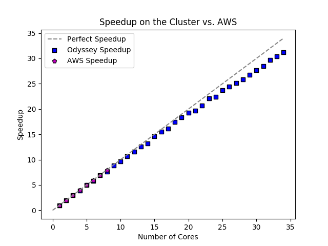
python plot_speedup.pyThe number of cores and partition can be modifies inrun.pyto generate more or less data for each run. We see a fantastic level of parallelization as number of cores increases using strong scaling. No significant deviation from perfect speedup appears until approximately 15 cores are used. Note, despite AWS speedup being comparable, AWS was approximately 50% slower for each calculation.
 Image generated from our 1792 x 2944 county matrix.
The main overheads here is distribution between threads. On Odyssey, the overhead of using OpenMP was negligible (and even tended to be faster than single thread calculations without). We see clearly, however, that this overhead is relatively insigificant when compared to the calculations being performed, as evidenced by the near perfect scaling until 15 cores.