CS205 Final Project
Cooper Lorsung • Sujay Thakur • Royce Yap • David Zheng
Big Data
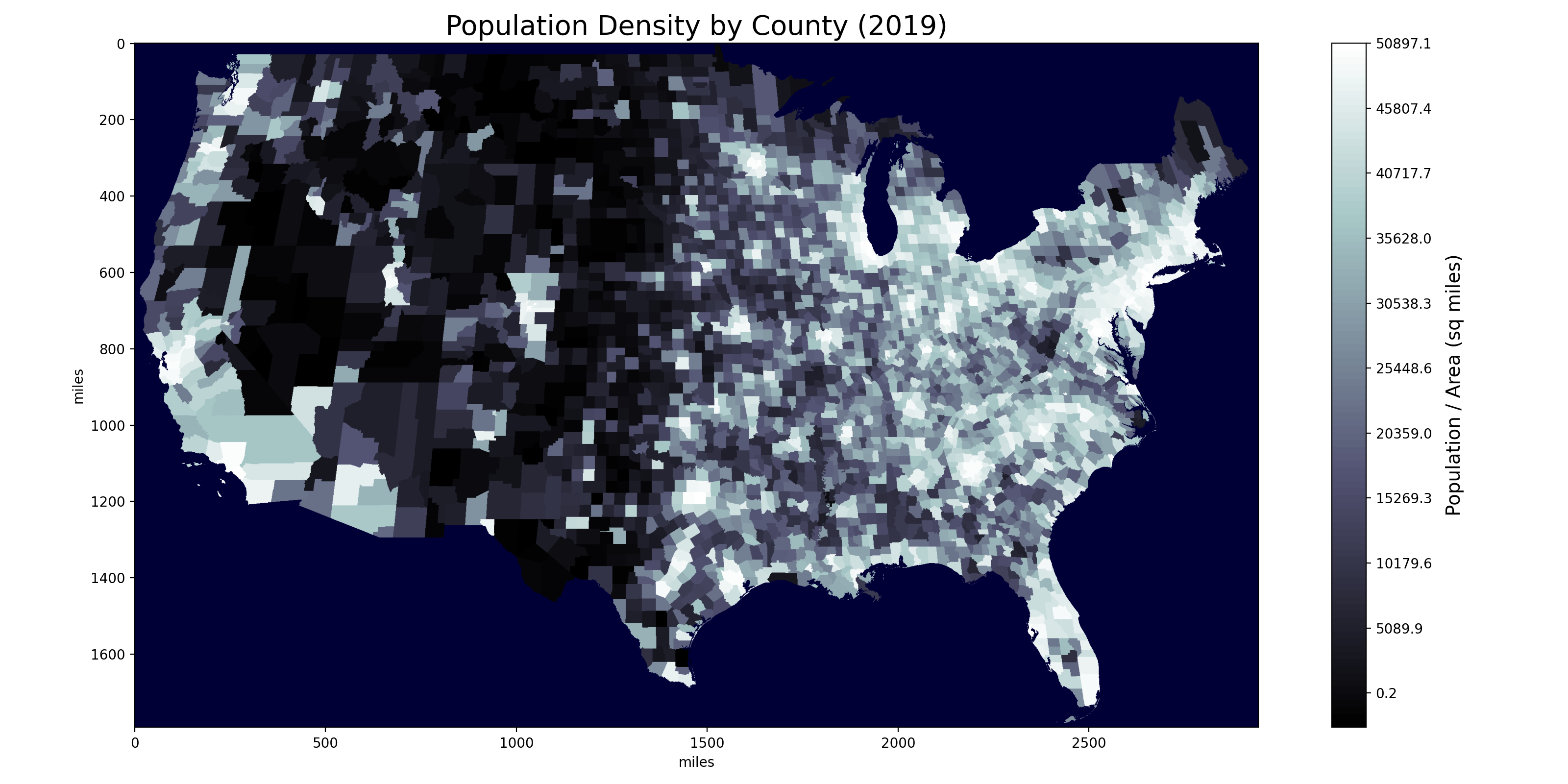
 Image generated from our 1792 x 2944 county matrix.
Mapping a Square-Mile Grid of the U.S. to County Data
To ensure that each square-mile of the 1792 x 2944 grid of continential U.S. takes in granular demographic information relating to that square-mile, we would need to map each square-mile to a particular county. Our goal is to create a matrix with each entry in the matrix corresponding to a county ID, that can be then mapped to specific data relating to the county (e.g. population) This information can then be used to generate matrices of β and γ values that can be fed into the SIR epidemic model.
Firstly, having realized that the earth is not flat, we had to use the Haversine formula to map each point in the 1792 x 2944 grid to a pair of coordinates corresponding to the latitude and longitude of that point.

Illustration of Haversine distances
This returned us a coordinate matrix of size 1792 (North-South distance) x 2944 (East-West Distance) x 2 (Latitude & Longitude), which we then had to map to U.S. counties by their FIPS (Federal Information Processing Standard) code.
Challenge
Here, the challenge that is solved by parallel application is that of determining which county a specific coordinate belongs to, based on its longitude and latitude. This is not as straightforward as it sounds and we were unable to find any prior existing work that had done such a mapping.
We obtained geographical information on U.S. counties from the Census’ TIGER Geodatabases. The geographical boundaries of every single county is captured in a shapefile format that can be read as a Polygon object by Geopandas.
Information from US Census data in a dataframe, with the last column containing cartographic boundaries
To verify if each pair of coordinates fell within the geographical boundary of a county, the within Geopandas method had to be used, since there is no pre-existing hash table mapping every single unique coordinate to a county. Only if the method returned the value “True” would we assign the coordinate to a particular GEOID.
The task to be completed then was to run through the 5,275,648 pairs of coordinates through the 3,233 unique GEOIDs in the file, representing a run-time complexity of O(m x n), where m is 5 million and n is 3,000.
The coordinate mapping returned 3108 unique FIPS codes across 3,121,073 coordinates, the remaining 2,154,575 coordinates were either non-US land or water. The returned FIPS codes exactly matched the 2019 US Census’s listing of counties in the continental United States and the District of Colombia.
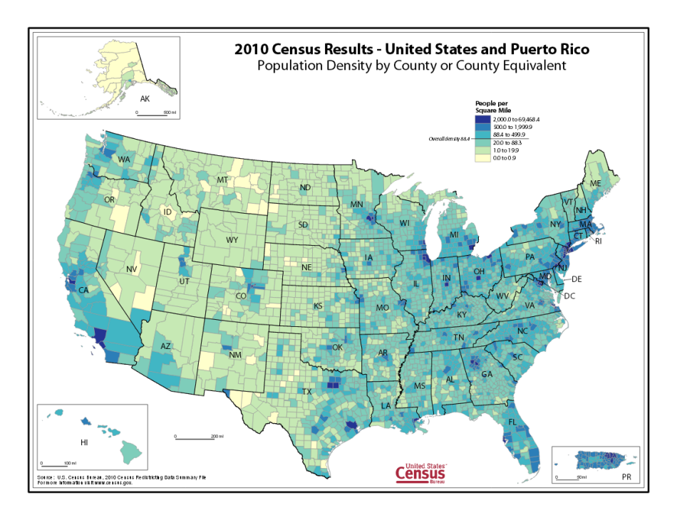
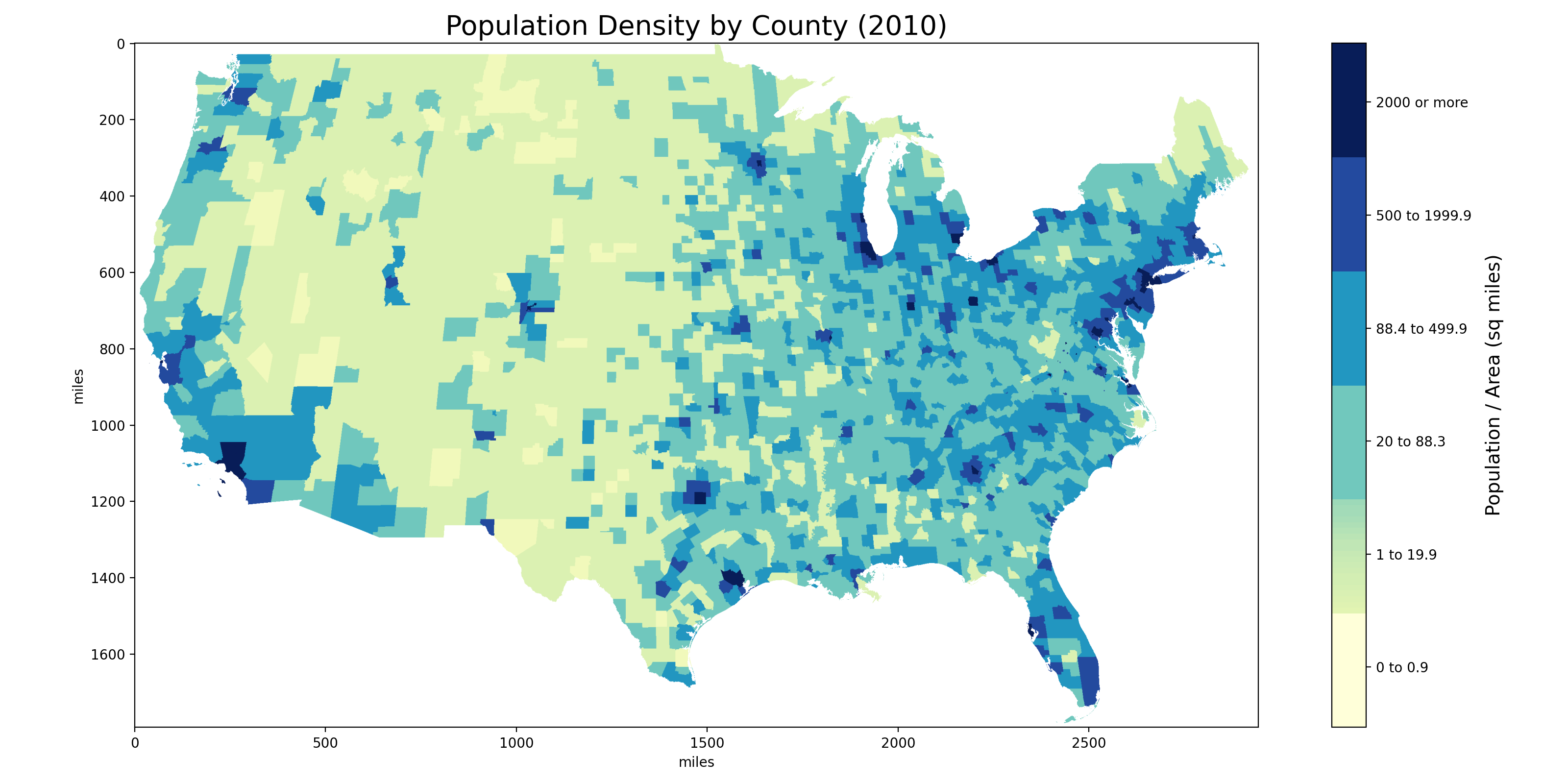
We furthur verified our results by visually inspecting plots of our matrix again excisting US county maps. For example, compare our mapping of population density against the official map from the US Census Bureau:
 US Census Map source
 Image generated from our 1792 x 2944 county matrix.
Description of Parallel Application
Parallelizing this application via Spark did not seem possible since the functions do not include the ability to work with geometry objects containing information on the boundaries of the counties.
To implement this parallel application on Hadoop, we used Geospark, which is a cluster computing system for processing large-scale spatial data. GeoSpark “extends Apache Spark / SparkSQL with a set of out-of-the-box Spatial Resilient Distributed Datasets (SRDDs)/ SpatialSQL that efficiently load, process, and analyze large-scale spatial data across machines”.

We used Amazon’s EMR cluster to provide the Hadoop infrastructure required for implementing our parallel application, with the following setup:
- Release label:emr-5.29.0
- Hadoop distribution:Amazon 2.8.5
- Applications:Spark 2.4.4
- Master Node: m4.2xlarge
- Worker Node: m4.xlarge (varying from 1 to 16 nodes)
Implementation of Spark / GeoSpark
First, after loading in a flattened matrix of coordinates as a Spark DataFrame, we use Spark SQL to create new column location with each location as a ST_POINT object containing each coordinate pair.
Next, we load in the Census Data on the counties and map the Polygon object in the geometry field to a WKT (well-known-text) format before converting it into a Spark DataFrame.
This comes the important step, where we implement the [ST_INTERSECTS method] (https://datasystemslab.github.io/GeoSpark/api/sql/GeoSparkSQL-Predicate/#st_intersects) in Spark SQL, which is key in allowing us to parallelize our lookup operation.
SQL code to determine point intersection in GeoSpark
We then merged data on the original coordinates with the mapped counties and converted this into a RDD format, which is then saved as a text file on the Hadoop File System. A sample output of the text file is shown below, where the first and second column represent the latitude/longitude, the third and fourth columns represent the row and column position in the matrix and the last column represents the county GEOID.
Sample GeoSpark Output
To put things in perspective, we processed 5,275,648 lines of the above using Spark.
Technical Description
To implement this required bootstrapping the AWS EMR cluster using a Bash script (link). Miniconda was used to install required packages across the nodes in the cluster, particularly because it handles the installation of GeoSpark and its dependencies.
Screenshot of Bash Script
The above script does the following:
- Downloads Miniconda
- Installs required packages (Geospark, Pandas, Geopandas, Haversine) across all nodes in the cluster
- Downloads Java ARchive (JAR) files required for GeoSpark onto EMR cluster
Separately, to ensure that GeoSpark runs smoothly, the configuration below also had to be added via a JSON when setting up the EMR cluster, to ensure that the JAR files are loaded when you creating a Spark instance.
Screenshot of EMR configuration
Lastly, the SPARK_HOME environment variables need to be set before running the Spark instance:
export SPARK_HOME=/usr/lib/spark
The following two lines are also added to /usr/lib/spark/conf/spark-env.sh:
export PYSPARK_PYTHON=/home/hadoop/conda/bin/python
export PYSPARK_DRIVER_PYTHON=/home/hadoop/conda/bin/python
Performance Evaluation
Our first attempt at implementing the county mapping operation using the multi-processing module on Python with 4 cores returned us with a run-time of 7 hours and 37 minutes.
Screenshot of Python runtime for mapping task
With Spark and Hadoop, we are talking about a completely different magnitude, with 130 seconds recorded as the fastest time with 16 m4.xlarge nodes, each with a supposed 4 cores.
Screenshot of GeoSpark runtime for mapping task
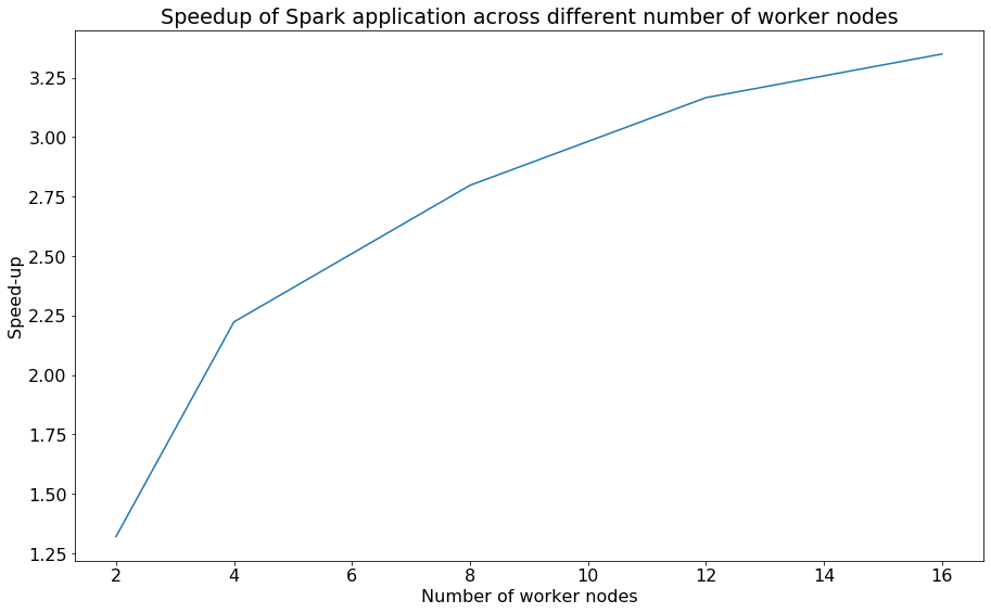
As shown below, by varying the number of worker nodes from 2, 4, 8, 12, 16, we are able to plot the speed-up of the Spark application which plateaus as it increases, with a single worker node taking 436 seconds or ~7 minutes.
 Speedup plot of Spark task
While we observe some version of Strong Scaling predicted by Amdahl’s Law, given the parallelization overheads undertaken by Spark in terms of communicating and synchronizing the data across the various nodes, it is expected that the speedup will plateau.
In fact, below, through the logs, we obtain a glimpse of how the YARN scheduler is killing some of the executors through the process, reducing the “new desired total” to below what we had provisioned for.
Log file showing YARN scheduler "killing" executors