Group 21 Spotify Project
Matthew Finney • Kaivalya Rawal • Royce Yap • David Zheng
k-NN User-Based Collaborative Filtering model
Overview
Given a given playlist of songs, assuming that users included songs that they deemed to be similar in the same playlist, we can predict songs in that playlist by finding a group of similar playlists to the input playlist and the songs that occur most frequently across these playlists.
Here, we can use a memory-based Collaborative Filtering model, which uses the k-NN algorithm to find k number of playlists that are most similar to our given playlist. There are two types of Collaborative Filtering models - User-Based and Item-Based. In the context of Spotify playlists, these translate to Playlist-Based vs. Song-Based (based on song features).
As informed by our EDA, songs in the same playlist do not necessarily share the same features. Our baseline model employed a version of the Item-Based approach, which returned a low level of prediction accuracy. Hence, here, we will go with the User-Based (Playlist-Based) Collaborative Filtering approach in predicting songs.
The similarity metric between playlists can be calculated using cosine distance, based on the co-occurence of songs in training set playlists and the target playlist. This is shown in the formula below, where A and B represent an array of track occurence in two playlists, Playlist A and Playlist B respectively.

The Playlist-Based Collaborative Filtering approach is playfully illustrated in the following image:
(Source: Spotify’s Recommendation Engine)
The higher the number of overlapping tracks between the playlists, the more similar they should be. Once these playlists have been identified, we then tabulate the frequency of songs that appear across these similar playlists and choose the top n-ranked songs as our recommended songs for the target playlist.
Preparation of Data
On the test set, which was randomly chosen from the full one million playlist dataset, we further split the data into a 70:30 split between the calibration set and withheld set, by stratifying by Playlist ID (“pid”). This is important in ensuring that a similar proportion of tracks in each playlist is fed into the model, to identify the similarity between the test playlists and the train playlists.
As part of preparing the data, we also checked on the proportion of songs in withheld list that is in training set. We obtained a 99%+ metric on this, which is an improvement over our baseline model which only had 100 training playlists and 20% of withheld songs in the training set. By ensuring sufficient overlap, this ensures that we are in a good starting position when making predictions.
An important step to note is that we also merged the calibration set together with the training set because the tracks in the calibration set are required in the binary sparse matrix that is fed into the k-NN model, to identify similar playlists.
Training the model
To train the model, we used the combined playlists with both the training and calibration data to create a matrix, with 14719 rows and 49855 columns. Each row represents a playlist and each column represents a song track. The individual values in row i and column j will represent whether the track is in the playlist (1) or not (0). Below shows the first few rows of the matrix, to give a better sense of what is being fed into the model:

We then used scipy Compressed Sparse Row matrix module to transform the matrix. This would allow for scalability as storage of numpy matrices tend to become infeasible as the matrix grows larger.
We then fit the Compressed Sparse Row matrix onto an unsupervised Nearest Neighbors learning model, where n_neighbors = 20 and cosine distance is used as a distance of measure. Here, we have set the neighbors search algorithm to auto, so that the algorithm attempts to determine the best approach from the training data across the options of BallTree, KDTree, and a brute-force algorithm.
Methodology - How the Model Makes Recommendations
Once we fitted the model, we had to create a separate method make_recommendations that would take in the Playlist ID and return a list of recommended tracks. Using the validation set, we fine-tuned number of neighbors as a parameter to identify the optimal number of neighbors that would return the highest score on the success metric.
Without going through the specific code, broadly, this is how it would work:
- Use the k-NN model to find the k nearest neighbors to the given Playlist ID, based on the calibration songs that were passed into the matrix
- For all the k nearest neighbor playlists found, create a frequency table of all the songs that appear in all the playlists
- Select the top songs from the frequency table and return a list of recommended songs as output
When we run the ‘make_recommendations’ method, it produces the following output of tracks for a given playlist.
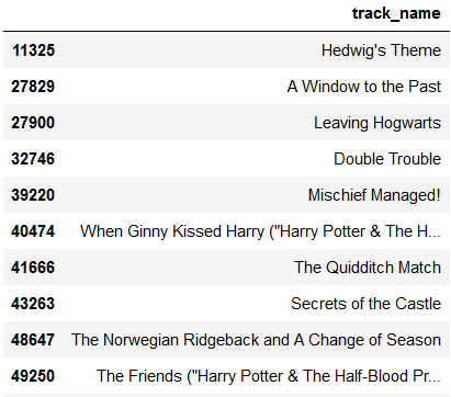
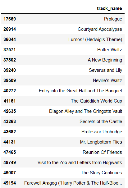
In this case, we did chance upon a Harry Potter playlist indeed and the predicted songs do come quite close to the songs that were withheld from the model, as shown below.
Validation - Fine-tuning n-neighbors parameter
As part of validation, we used 10, 25, 50 as the number of neighbors as parameters to be fed into the model. We capped the number of neighbors at 50, to limit the run-time of the model. Unsurprisingly, having 50 neighbors returns the highest R-Precision Score (RPS) and Normalized Discounted Cumulative Gain (NDCG) scores. This makes intuitive sense, given that by going through a larger list of neighbors, we are likely to converge on the tracks with the highest frequencies.
The table below shows the result on the validation set, based on the metrics of R-Precision Score (RPS) and Normalized Discounted Cumulative Gain (NDCG):

Model Performance
We have identified the three metrics (RPS, NDCG and hit-rate) to evaluate our model. To obtain the final metrics, we compute the mean of the scores across all the playlists in the test set, across different values for number of recommendations.
Below the histograms show a distribution of the scores across the three different metrics, with two distributions for RPS and NDCG, one each for the case where the number of recommendations equals the number of songs used for calibration and where it equals the number of withheld songs.

Overall, with 50 neighbors, the k-NN collaborative filtering model achieved a 0.313 R-precision score and 0.249 NDCG score by producing the same number of recommendations as the number of songs used to calibrate the model. The R-precision score of 0.313 implies that if given a list of 100 songs, the model is able to produce 100 songs, out of which 31.3 on average would be songs that were in the withheld list of songs.
Discussion
In the k-NN Collaborative Filtering model, we only consider track co-occurence between playlists and assign a 1 or 0 based on its occurence in the playlist. Going forward, if we are able to obtain ratings on how well a song fits a playlist, this could be fed into the matrix used for the k-NN model and hence, improve our ability to predict songs that are likely to be in a playlist.